EfficientNet: Rethinking Model Scaling for Convolutional Neural Networks

1. Abstract

• Scaling network depth, width and resolution leads to better performing model.
• However, choosing scaling value and which component to scale can be problematic.
• This paper proposes new scaling method that uniformly scale detph, width and resolution by using compound coefficient

2. Introduction

• Scaling ConvNets is done in various ways, but the most common way is to scale up by their depth, width and resolution.

• In previous work, scaling only one of these three components has been done, for scaling two or three dimensions requires tedious manual tuning with lots of resources.

• However, it is possible to balance all dimensions of network width, depth and resolution by scaling each of them with constant ratio. This process is called compound scaling method.

3. Compound Model Scaling

3.1. Problem Formulation

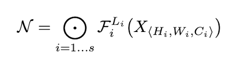
• ConvNet layer i can be defined as following function.

$Y_i = F_i(X_i)$

• $Y_i$ is output tensor, $F_i$ is operator and $X_i$ is input data with a shape of [$H_i, W_i, C_i$], where $H_i$ and $W_i$ are image height and width and $C_i$ is number of channels.

• Therefore, the whole ConvNet is defined as follows:

$N = F_1 * F_2 * F_3 * … * F_k$

• ConvNets are usually partitioned into multiple stages and all layers in each stage share same architecture. Therefore, ConvNet can be defined in different way:

• $F_i^{L_i}$ denotes layer $F_i$ is repeated $L_i$ times in stage i.

• Model scaling tries to expand network depth($L_i$), width($C_i$) and resolution($H_i, W_i$), without changing the predefined architecture $F_i$.

• The goal of this network is trying to achieve target memory and target Flops by scaling with constant ratio. Such process is formulated as follows:

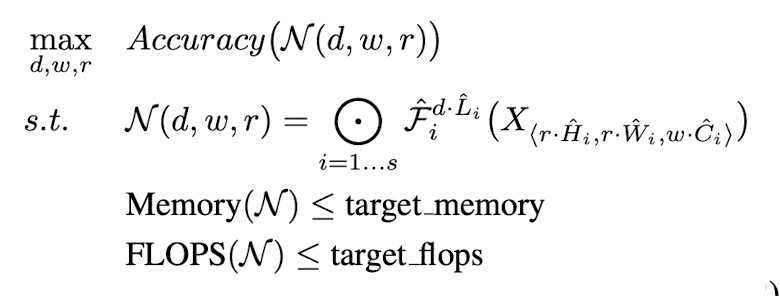
• $w, d, r$ are coefficient for scaling network width, depth, and resolution.

3.2 Scaling Dimensions

This section shows accuracy changes when scaling one of these dimensions is done.

Depth($d$)

• Pros: Deeper network can capture richer and more complex features, and works generally well for new tasks.
• Cons: Accuracy gain decreases due to vanishing gradient problem.
• Solution: skip connection, batch normalization

Width($w$)

• Pros: Wider network tends to capture more fine-grained features and easier to train, due to small size of the model.
• Cons: Wide but shallow networks tends to have difficulties in finding higher level features.

Resolution($r$)

• Pros: With higher resolution input image, ConvNet can capture more fine-grained patterns.
• Cons: Accuracy gain diminishes for very high resolutions.

Conclusion: Scaling one of these dimensions improves accuracy, but its gain decreases as the model gets bigger.

3.3 Compound Scaling

• Scaling dimensions are not independent to each other. For example, when image resolution gets higher, network should be wider to capture more fine-grained patterns. Therefore, multiple dimensions should be scaled simultaneously rather than conventional single dimension scaling.

• This paper proposes compound scaling method, which use a compound coefficient $\phi$ to uniformly scale all dimensions:

depth: $d = \alpha^\phi$ width: $w = \beta^\phi$ resolution: $r = \gamma^\phi$

• $\phi$ denotes user-specified coefficient which is controlled by avaliable resources.

• $\alpha, \beta, \gamma$ denotes constants that can be determined by grid search.

• Total FLOPS is increased by ($\alpha * \beta^2 * \gamma^2$)

4. EfficientNet Architecture

• Since model scaling does not change the overall architecture $F_i$, having a good baseline network is crucial.

• Neural architecture search is utilized to optimize both accuracy and FLOPS. The search result is named EfficientNet-B0 and the architecture looks as follows:

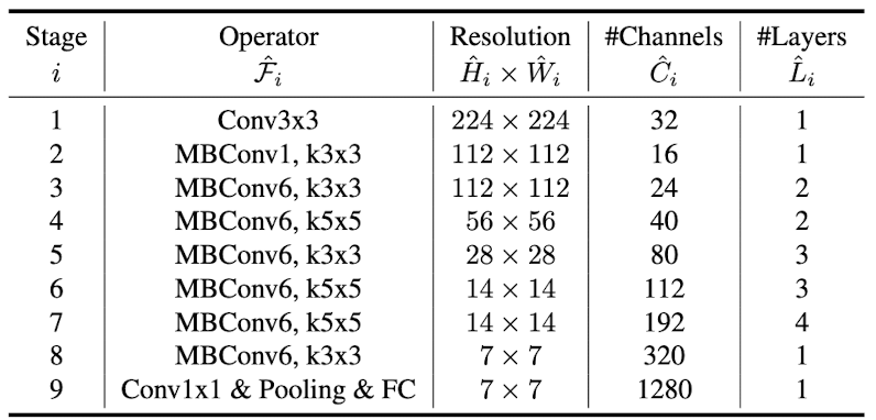
• Starting from the baseline network EfficientNet-B0, compound scaling method is divided into two steps:

Step 1: Fix $\phi = 1$, and do the grid search to find best values for $\alpha, \beta, \gamma$. The results are $\alpha = 1.2, \beta = 1.1, \gamma = 1.15$, under the constraint of $\alpha * \beta^2 * \gamma^2 \approx 2$

Step 2: Fix $\alpha, \beta, \gamma$ as constant, and adjust $\phi$ with different values to make EfficientNet-B1 to B7.

5. Experiments

5.1 Scaling Up MobileNets and ResNets

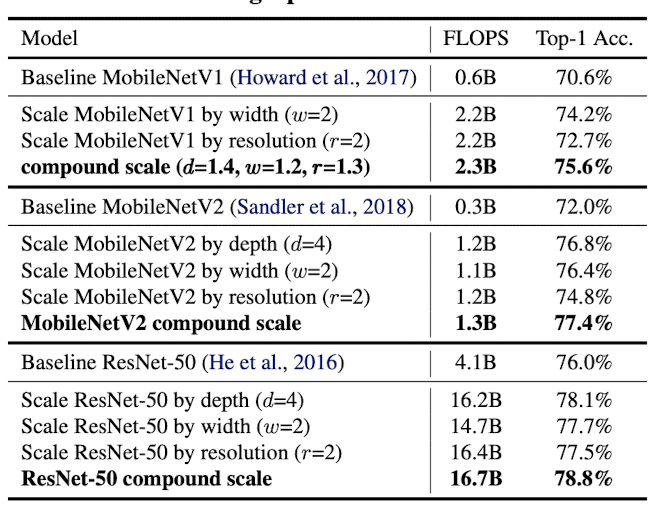
• Compound scaling method is first applied to widely-used MobileNets and ResNet. Scaled models both show significant accuracy improvement compared to previous models.

5.2 ImageNet Results for EfficientNet

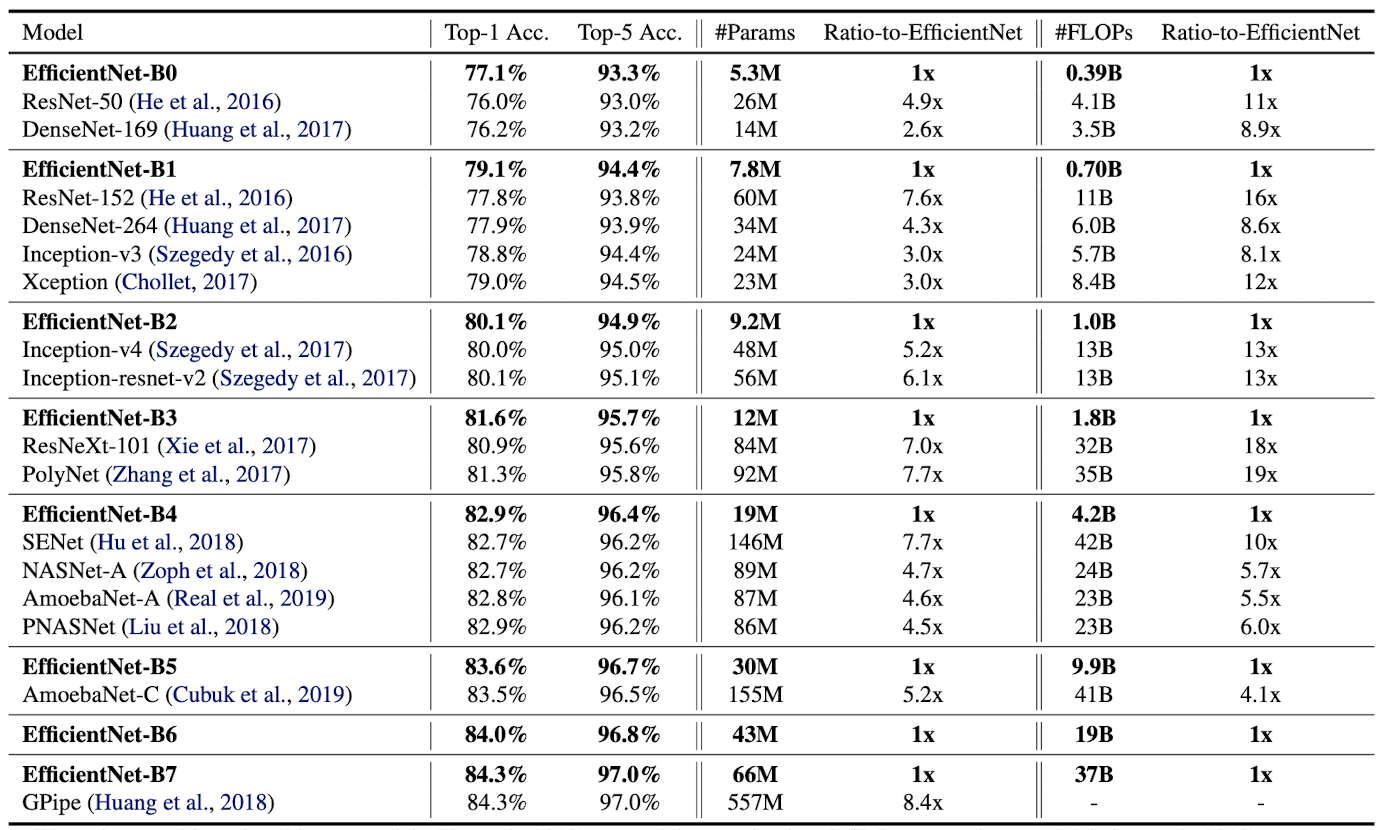
• Scaling method is then applied to EfficientNet models. Number of parameters and FLOPs are both significantly lower than existing ConvNets, while accuracy is either similar or higher.

• Latency is also measuered for EfficientNet-B1 and EfficeintNet-B7, and both run about 6 times faster than ResNet-152 and GPipe. This implies that EfficientNets are fast on real hardware.

5.3 Transfer Learning Results for EfficientNet

• EfficientNet is also evaluated on transfer learning dataset. Compared to other models with similar accuracy, EfficientNet show significantly less parameters.

6. Discussion

• To discover the effect of compound scaling, ImageNet performance of different scaling method for the same EfficientNet-B0 has been compared. All scaling methods improve accuracy with the cost of more FLOPS, but compound scaling can further improve accuracy by up to 2.5%.

7. Conclusion

• Compound model scaling, which scales the dimension of depth, width and resolution by constant ratio, highly saves resources while maintaining its performance.