Learning Intra-Batch Connections for Deep Metric Learning

1. Introduction

• Metric learning is a techinque which takes the input image and scale it down to more compact, embedding space. In that embedding space, samples with same class should be closer than the ones with different classes.

• Various loss functions were used to map the input data into embedding space. Contrastive loss minimizes the distance between positive pair while maximizing the distance otherwise. Triplet loss takes the triplet of images and pushes the anchor to be closer to the positive sample than the negative one.

• The problem around contrastive loss and triplet loss is that the vast majority of pairs (or triplets) are not important enough to contribute to the loss. In other words, it is important for loss functions to consider the global structure of the dataset and update the loss regarding that matter. Contextual classification loss functions and Group loss are the recent works that addresses this problem, but the global structure is captured using a handcrafted rule instead of learning.

• The model proposed in this paper utilizes MPN(Message Passing Network) to allow the samples in a mini-batch to communicate with each other. More specifically, the input samples are the results of the images passed into CNN(Convolutional Neural Network).

2. Related Work

1. Metric Learning Losses: Metric learning loss includes contrastive loss and triplet loss. N-pair loss is the recent work where an anchor and a positive samples are compared to N-1 negative samples at the same time.

2. Sampling and Ensembles: Since not all data are informative, intelligent sampling is introduced to better sample the necessary data. At the same time, ensembling technique was applied to metric learning, and showed better result than the single network trained on the same loss.

3. Global Metric Learning Losses: Global metric learning losses utilizes proxy data points, which approximates original data points so that a triplet loss over the proxies is a tight upper bound of the loss over original samples.

4. Classification Losses for Metric Learning: It is shown that a carefully designed classification loss function can outperform triplet-based functions in metric learning. One exmaple, SoftTriple loss develops a classification loss where each class is represented by K centers. Other example, Group Loss replaces softmax function with other contextual module, considering all the samples in the mini batch at the same time.

5. Message Passing Networks: The main idea of this network is that not only the embeded nodes and edges are considered, but also those of the neighbors in the graph, as well as the overall graph topology. This network have revolutionized the field of NLP(Neural Language Processing) and Computer Vision, especially object detection.

3. Methodology

3.1 Overview

The proposed method works as following step:

1. Embed the image into higher dimension using CNN and fully connected graph.
2. Pass through message passing network to refine the initial embedding feature vectors by using dot-prodcut self attention.
3. Perform classification and optimize both the MPN and backbone CNN using cross entropy loss.

3.2 Feature Initialization and Graph Construction

The global structure of the embedding space is formulated by following graph:

$\gamma = (V, E)$

• $V$ represents the nodes. In other words, they are the images passed to the network
• $E$ represents edges, which connects nodes showing the importance of each edges to others.
• Since considering all the data into account takes huge amount of resource computationally, mini-batches consisting of $n$ randomly sampled class with $p$ randomly chosen samples per class is considered.
• Then the MPN is structured to make relations between mini-batches.
• CNN is used for embeddings.

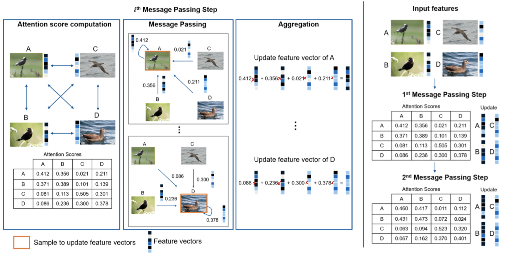
3.3 Message Passing Network

Message Passing Network is applied to embeddings to exchange information between mini-batches. The message passing process is formulated as follows:

$h_i^{l+1} = \sum_{j\in N_i}W^{l}h_j^{l}$

• $h_i^{l+1}$ is an updated feature of node $i$ at step $l+1$.
• $h_j^{l}$ is features of neighboring node $i$ at step $l$.
• $W^{l}$ is the weight matrix of message between node $i$ and its neighboring node $j$.

As stated in introduction section, not all samples are important for updating decision boundary between classes. Therefore, attention score, $\alpha$ is added to every message passing step to weigh importance of each samples to other samples.

$h_i^{l+1} = \sum_{j\in N_i}\alpha_{ij}^{i}W^{l}h_j^{l}$

• $\alpha_{ij}^{i}$ is the attention score between node $i$ and $j$.

Skip connection is then applied to the attention block, $f(h_{i}^{l+1})$. This step is formulated as follows:

Step 1: $f(h_{i}^{l+1}) = LayerNorm(h_{i}^{l+1} + h_{i}^{l}))$
Step 2: $g(h_{i}^{l+1}) = LayerNorm(FF(f(h_{i}^{l+1})) + f(h_{i}^{l+1}))$

• F stands for fully connected layer. Therefore, FF represents two fully connected layers.
• Result after normalization, $g(h_{i}^{l+1})$, is then passed to the next message passing step.

Below illustration shows how the attention score makes the image coming from the same class closer while the opposite further as the message passing steps progress.

3.4 Optimization

Fully connected layer is applied after the last message passing step and cross entropy loss is used to classify. Since the last cross entropy loss is not used during test time, auxiliary cross entropy loss is also applied to the backbone CNN.

3.5 Inference

The experiments done to test the performance of the model do not use the last cross entropy loss because MPN requires batch of samples.

4. Experiments

4.1 Implementation details

1. Backbone CNN model: ResNet50 pretrained on ILSVRC 2012-CLS dataset
2. Preprocessing: Resized the cropped images to 224x224 during train time, and resized the images to 256x256 and take a center crop of size 227x227 during test time.
3. Training parameters: Train all networks for 70 epochs using RAdam optimizer
4. Evaluation metrics: Two commonly used evaluation metrics were used
   • Recall@K : Evaluates the retrieval performance by computing the percentage of images whose K nearest neighbors contain at least one sample of the same class as the query image.
   • NMI: Evaluates how much the knowledge about the ground truth classes increases given the clustering obtained by the K-means algorithm.

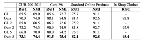
4.2 Comparison to state-of-the-art

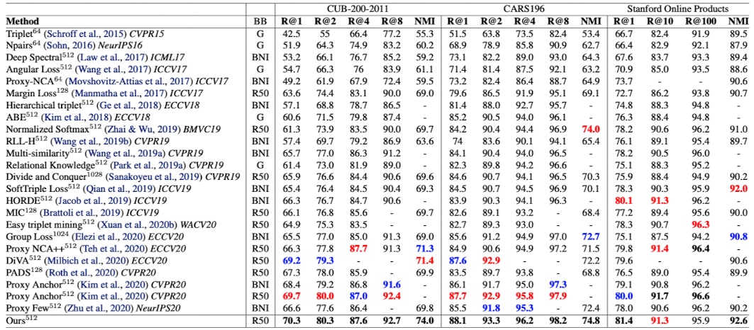
• Bold number indicates the best result, Red indicates the second best result and Blue indicates the third best result.
• The model proposed in this paper achieves state-of-the-art performance, scoring higher than all the current best methods.

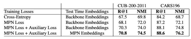
4.3 Ablation Studies and Robustness Analysis

1. Adding auxiliary loss function (cross-entropy loss) at the top of the backbone CNN improves the performance of overall model.

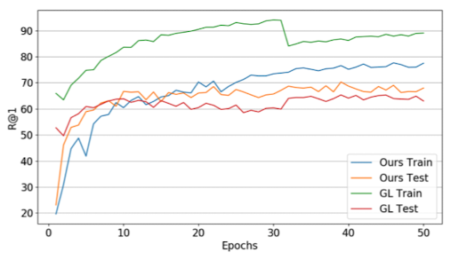
2. When compared to model with Group Loss, model with MPN shows less overfitness and better test result.

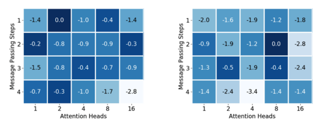
3. Experiment was conducted to find out the best number of message passing steps and attention heads of MPN. The numbers show the relative difference to the best model. Therefore, the combination marked with 0.0 is the parameter that shows the best result.

4. Since Group Loss shows the performance increase by using an ensemble at test time, experiment was conducted on MPN ensembles using 2 and 5 networks. In all cases, MPN ensembles show better result than Group Loss ensembles.

Conclusion

1. This paper proposes new model that utilizes all intra-batch relations in the mini-batch to promote similar embeddings for images coming from the same class, and dissimilar embeddings for images coming from different classes.

2. This new model performs better than all the current best method, while using same number of parameters